| 
Creating Gantt Charts in Excel using Integra
Excel does not contain a built-in Gantt chart format; however, you can easily create a Gantt chart in Excel by customizing the stacked bar chart type. In this FAQ we show you an example on how to create a Gantt Chart. Populating the data in Excel from your Notes data is done in the usual manner.
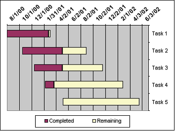
This FAQ shows you how to create a Gantt chart like the following example.

 Step 1: Enter the sample data Step 1: Enter the sample data
1. Open a new worksheet in Excel and enter the following values in cells A1 through D6:
 | A | B | C | D |
1 |  | Start Date | Completed | Remaining |
2 | Task 1 | 08/01/2000 | 205 | 10 |
3 | Task 2 | 10/15/2000 | 200 | 120 |
4 | Task 3 | 12/15/2000 | 140 | 200 |
5 | Task 4 | 02/06/01 | 44 | 345 |
6 | Task 5 | 05/06/01 | 0 | 380 |
Note The values in columns C and D (Completed and Remaining) represent numbers of days.
2. Select cell B2 and format with the date format you want to use for the chart by clicking Cells on the Format menu, and then clicking the Number tab. Click Date in the Category list, and select the format you want to use in the Type list.  Step 2: Create a stacked bar chart Step 2: Create a stacked bar chart
1. Select cells A1:D6 and click Chart Wizard.
2. In step 1, click Bar under Chart Type, and then click the Stacked Bar sub-type (you can see the name of each chart sub-type at the bottom of the dialog box).
3. Click Next, Next, and then Finish.
 Step 3: Make the chart look like a Gantt chart Step 3: Make the chart look like a Gantt chart
1. Double-click the first series in the chart. This is the series for Start Date. If default colors are set in Excel, this series is blue.
2. On the Patterns tab of the Format Data Series dialog box, click None for Border and None for Area, and then click OK.
3. Double-click the category (x) axis, which in a bar chart is the vertical axis. (In a bar chart, the traditional x and y axes are reversed.) Click the Scale tab, and select the Categories in reverse order check box.
4. Click the Font tab, click 8 under Size, and then click OK.
5. Double-click the value (y) axis, which in a bar chart is the horizontal axis. After completing the last step, this axis should be located at the top of the chart plot area. Click the Scale tab and type the following values in the appropriate boxes:
Minimum: 36739
Maximum: 37441
Major unit: 61
Minor unit: 1
These values are serial numbers that represent the dates to be used for the value (y) axis. The minimum value 36739 represents the date August 1, 2000. The maximum value 37441 represents the date July 4, 2002. The major unit of 61 represents about two months, while the minor unit represents one day. To see the serial number for a date, enter the date in a cell, and then format that cell with the General number format.
6. Also on the Scale tab, select the Category (X) axis crosses at maximum value check box.
7. Click the Alignment tab, and under Orientation, type 45 in the Degrees box.
8. Click the Font tab, and under Font style, click Bold. Under Size, click 8, and then click OK.
9. Right-click the legend, and click Format Legend on the shortcut menu.
10. Click the Placement tab, and click Bottom.
11. Within the legend, click Start Date so that it is selected, and then press DELETE.
After completing these steps, you should have a chart that looks similar to the example shown above. You may need to resize the chart using the mouse to see all of the labels present in the chart. Additional formatting can be added as needed.
When setting up the template for Integra to populate the spreadsheet, you create the Gantt Chart with ficticious data and when the formatting is to your liking, you clear the data_block and save the template. When Integra runs, it will populate your Gantt Chart right away..
We also refer you to an FAQ which explains how to automatically trigger the running of a Macro inside Excel from Integra | 
. |